A common goal in evolutionary biology is to understand how selection acts on traits and how genetic variants associated with those traits are affected by selection. The effect of selection on the genome is particularly interesting because there are situations where we know that populations are likely under different selection pressures (for example, one population of fish lives in freshwater and the other lives in saltwater), but the exact traits that selection is acting on may not be known or measurable. In the freshwater-saltwater fish example, the relevant trait experiencing selection pressure may be related to the ability for the gills to extract oxygen from the water – but measuring that might be tricky. So, researchers turn to the genome to attempt to understand how selection is acting on populations.
A basic distinction can be made between directional and balancing selection – is selection favoring one particular trait within the population (directional selection) or is selection favoring a mix of traits (balancing selection). To return to the freshwater-saltwater fish example, you might think that directional selection is most likely to be involved, because the freshwater and saltwater environments are incredibly different. But what if the freshwater environment is really a brackish environment that experiences fluctuations of low-salinity? Then perhaps the population will maintain variation among individuals in their ability to extract oxygen from the water because of variation in the micro-climate or temporally fluctuating conditions.
At the genetic level, the difference between directional and balancing selection can be thought of in this way: under directional selection, the populations will likely diverge, so the loci experiencing the effects of selection will have different allele frequencies (high FST between populations). However, directional selection will also erode genetic diversity (each population will tend towards only having one allele). With balancing selection, genetic diversity will be maintained (there will be many alleles in the populations) so the populations won’t diverge very much (low FST between populations).
A common approach to detecting these differences was proposed by Beaumont and Nichols in 1996, which it essentially identifies loci that have extreme FST values relative to their expected heterozygosity (which is a way of measuring their genetic diversity) by comparing the actual data to a simulated dataset with similar sampling parameters. This method then identifies loci that are under directional vs balancing selection by comparing FST values based on how much genetic diversity is expected for each locus. The simulations that are used to identify which loci are more extreme than expected (and therefore likely to be experiencing selection) are based on the infinite island model, which is a model of migration that assumes that there are infinite islands from which migrants arise. Although this is an abstraction from reality, Beaumont and Nichols showed that as long as a large number of independent populations are sampled (>10), the abstraction doesn’t skew the results very much. The Beaumont and Nichols (1996) approach has been widely used, especially since it has been developed into a user-friendly program called LOSITAN (Antao et al. 2008).
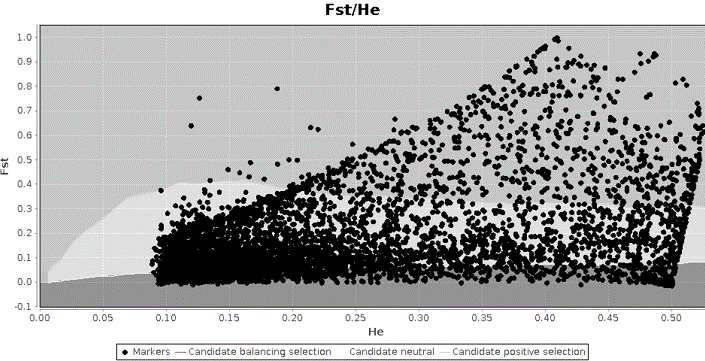
However, when I was conducting my population genomics study, I ran my data in LOSITAN and found some surprising results. I had sampled 12 populations, so I thought I should have enough samples, but I ended up with this graph:
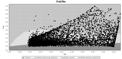
My pipefish genomic data analyzed by LOSITAN. The light grey area in the middle background is the region that is supposedly full of neutral loci, and the darker grey areas represent areas under balancing selection (bottom – darkest grey) and under directional selection (top – medium grey).
This graph was surprising because it identified hundreds of loci as being under selection, and it looked disturbingly skewed. For comparison, the figure below is from a study of lamprey populations by Hess and colleagues (2012), and shows what an expected distribution should look like:
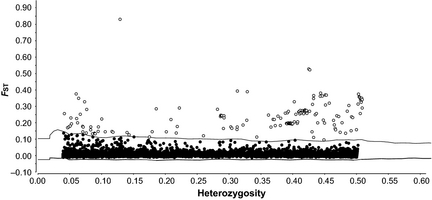
Genetic data from lamprey. Figure from Hess et al (2012), published in Molecular Ecology – not my own! Copyright held by Hess et al (2012)
My PhD advisor (Adam Jones) and I decided to investigate whether this skewed pattern was a symptom of a larger problem in our dataset or whether it was a common pattern in the literature. We found that the majority of studies reporting figures from LOSITAN analyses have unexpected patterns. Using simulations, we found that these patterns are caused by the relationship between FST and expected heterozygosity (FST is calculated using the expected heterozygosity), and that the skewed patterns like the one I found occur primarily when few independent populations are sampled, especially when migration rates are low between them. The skewed patterns are not a problem, per se, as they do result from a mathematical constraint between FST and heterozygosity. However, the confidence intervals used to identify putatively selected loci do not align with the actual patterns, leading to an excess of outlier loci – and therefore those outliers are not as reliable as candidate genes of interest. The results of these analyses have just been published in the Journal of Heredity
But wait, you might be thinking, didn’t you sample 12 populations? Good memory! Yes, I did. However, those populations clustered into larger clusters, due to isolation by distance, suggesting that they may not be truly independent. Therefore, the FST-heterozygosity distribution of my data reflects more closely the distribution of a sample from only 3 or 4 populations.
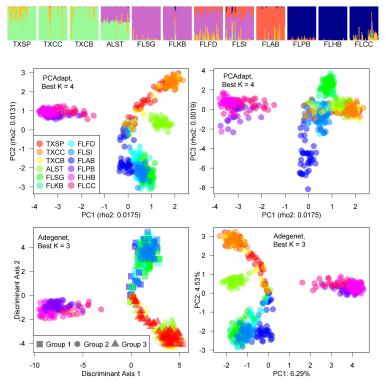
Genetic groupings: the populations sort into 3-4 groups (Flanagan et al. 2016)
So what do my recent results mean for researchers? First, be aware of the assumptions underlying the analysis methods you’re using! I was incredibly surprised by the number of studies that found an odd or skewed pattern that also didn’t meet the specified requirements (>10 populations). Second, if your study doesn’t fit the assumptions of the models you’re using, it may be best not to use that model! I was also amazed that no other researchers had mentioned the skewed Fst-heterozygosity relationship in their papers! Of the 112 papers presenting LOSITAN figures, 87 of them likely have an excess of outlier loci. This will affect inferences regarding the signature of selection as well as the future use of those loci as potential candidate regions for targeted studies. If people really want to use the Fst-heterozygosity comparison, especially if their dataset is only a little skewed, I have developed an R package called fsthet that will allow you to identify loci using quantiles drawn from the distribution of your data (rather than from simulations with model assumptions). This has its own drawbacks but might be useful for some people. Finally, using multiple approaches may help identify when an analysis isn’t right for your dataset. – one of the reasons the LOSITAN results stood out to me was because it identified so many more ‘significant’ loci than the other analyses I did. To summarize: think critically about your data, your analyses, and your results.
References (with links)

[…] emerging from analytical roadblocks is a theme for some of my recent papers, as I describe in these previous posts). I found that, although I could run the traditional parentage analysis program CERVUS on […]